Neural Network tutorial

Introduction

There is vast literature on neural networks and their uses, as well as strategies for choosing initial points effectively, keeping the algorithm from converging in local minima, choosing the best model structure, choosing the best optimizers, and so forth. mlpack implements many of these building blocks, making it very easy to create different neural networks in a modular way.

mlpack currently implements two easy-to-use forms of neural networks: Feed-Forward Networks (this includes convolutional neural networks) and Recurrent Neural Networks.

Table of Contents

This tutorial is split into the following sections:

• Introduction
• Table of Contents
• Model API
• Layer API
• Model Setup & Training
• Saving & Loading
• Extracting Parameters
• Further documentation

Model API

There are two main neural network classes that are meant to be used as container for neural network layers that mlpack implements; each class is suited to a different setting:

• FFN: the Feed Forward Network model provides a means to plug layers together in a feed-forward fully connected manner. This is the 'standard' type of deep learning model, and includes convolutional neural networks (CNNs).
• RNN: the Recurrent Neural Network model provides a means to consider successive calls to forward as different time-steps in a sequence. This is often used for time sequence modeling tasks, such as predicting the next character in a sequence.

Below is some basic guidance on what should be used. Note that the question of "which algorithm should be used" is a very difficult question to answer, so the guidance below is just that—guidance—and may not be right for a particular problem.

• Feed-forward Networks allow signals or inputs to travel one way only. There is no feedback within the network; for instance, the output of any layer does only affect the upcoming layer. That makes Feed-Forward Networks straightforward and very effective. They are extensively used in pattern recognition and are ideally suitable for modeling relationships between a set of input and one or more output variables.
• Recurrent Networks allow signals or inputs to travel in both directions by introducing loops in the network. Computations derived from earlier inputs are fed back into the network, which gives the recurrent network some kind of memory. RNNs are currently being used for all kinds of sequential tasks; for instance, time series prediction, sequence labeling, and sequence classification.

In order to facilitate consistent implementations, the FFN and RNN classes have a number of methods in common:

• Train(): trains the initialized model on the given input data. Optionally an optimizer object can be passed to control the optimization process.
• Predict(): predicts the responses to a given set of predictors. Note the responses will reflect the output of the specified output layer.
• Add(): this method can be used to add a layer to the model.

Note

To be able to optimize the network, both classes implement the OptimizerFunction API. In short, the FNN and RNN class implement two methods: Evaluate() and Gradient(). This enables the optimization given some learner and some performance measure.

Similar to the existing layer infrastructure, the FFN and RNN classes are very extensible, having the following template arguments; which can be modified to change the behavior of the network:

• OutputLayerType: this type defines the output layer used to evaluate the network; by default, NegativeLogLikelihood is used.
• InitializationRuleType: this type defines the method by which initial parameters are set; by default, RandomInitialization is used.

template<
  typename OutputLayerType = NegativeLogLikelihood<>,
  typename InitializationRuleType = RandomInitialization
>
class FNN;

Internally, the FFN and RNN class keeps an instantiated OutputLayerType class (which can be given in the constructor). This is useful for using different loss functions like the Negative-Log-Likelihood function or the VRClassReward function, which takes an optional score parameter. Therefore, you can write a non-static OutputLayerType class and use it seamlessly in combination with the FNN and RNN class. The same applies to the InitializationRuleType template parameter.

By choosing different components for each of these template classes in conjunction with the Add() method, a very arbitrary network object can be constructed.

Below are several examples of how the FNN and RNN classes might be used. The first examples focus on the FNN class, and the last shows how the RNN class can be used.

The simplest way to use the FNN<> class is to pass in a dataset with the corresponding labels, and receive the classification in return. Note that the dataset must be column-major – that is, one column corresponds to one point. See the matrices guide for more information.

The code below builds a simple feed-forward network with the default options, then queries for the assignments for every point in the queries matrix.

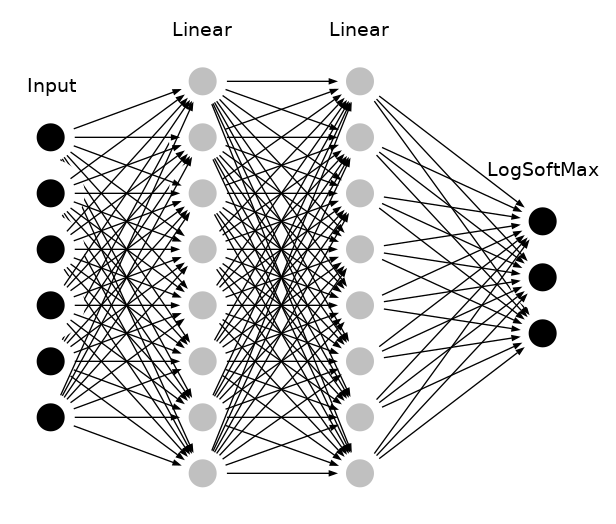
Note

The number of inputs in the above graph doesn't match with the real number of features in the thyroid dataset and are just used as an abstract representation.

#include <mlpack/core.hpp>
#include <mlpack/methods/ann/layer/layer.hpp>
#include <mlpack/methods/ann/ffn.hpp>

using namespace mlpack;
using namespace mlpack::ann;

int main()
{
  // Load the training set and testing set.
  arma::mat trainData;
  data::Load("thyroid_train.csv", trainData, true);
  arma::mat testData;
  data::Load("thyroid_test.csv", testData, true);

  // Split the labels from the training set and testing set respectively.
  // Decrement the labels by 1, so they are in the range 0 to (numClasses - 1).
  arma::mat trainLabels = trainData.row(trainData.n_rows - 1) - 1;
  arma::mat testLabels = testData.row(testData.n_rows - 1) - 1;
  trainData.shed_row(trainData.n_rows - 1);
  testData.shed_row(testData.n_rows - 1);

  // Initialize the network.
  FFN<> model;
  model.Add<Linear<> >(trainData.n_rows, 8);
  model.Add<SigmoidLayer<> >();
  model.Add<Linear<> >(8, 3);
  model.Add<LogSoftMax<> >();

  // Train the model.
  model.Train(trainData, trainLabels);

  // Use the Predict method to get the predictions.
  arma::mat predictionTemp;
  model.Predict(testData, predictionTemp);

  /*
    Since the predictionsTemp is of dimensions (3 x number_of_data_points)
    with continuous values, we first need to reduce it to a dimension of
    (1 x number_of_data_points) with scalar values, to be able to compare with
    testLabels.

    The first step towards doing this is to create a matrix of zeros with the
    desired dimensions (1 x number_of_data_points).

    In predictionsTemp, the 3 dimensions for each data point correspond to the
    probabilities of belonging to the three possible classes.
  */
  arma::mat prediction = arma::zeros<arma::mat>(1, predictionTemp.n_cols);

  // Find index of max prediction for each data point and store in "prediction"
  for (size_t i = 0; i < predictionTemp.n_cols; ++i)
  {
    prediction(i) = arma::as_scalar(arma::find(
        arma::max(predictionTemp.col(i)) == predictionTemp.col(i), 1));
  }

  /*
    Compute the error between predictions and testLabels,
    now that we have the desired predictions.
  */
  size_t correct = arma::accu(prediction == testLabels);
  double classificationError = 1 - double(correct) / testData.n_cols;

  // Print out the classification error for the testing dataset.
  std::cout << "Classification Error for the Test set: " << classificationError << std::endl;
  return 0;
}

Now, the matrix prediction holds the classification of each point in the dataset. Subsequently, we find the classification error by comparing it with testLabels.

In the next example, we create simple noisy sine sequences, which are trained later on, using the RNN class in the RNNModel() method.

void GenerateNoisySines(arma::mat& data,
                        arma::mat& labels,
                        const size_t points,
                        const size_t sequences,
                        const double noise = 0.3)
{
  arma::colvec x =  arma::linspace<arma::Col<double>>(0,
      points - 1, points) / points * 20.0;
  arma::colvec y1 = arma::sin(x + arma::as_scalar(arma::randu(1)) * 3.0);
  arma::colvec y2 = arma::sin(x / 2.0 + arma::as_scalar(arma::randu(1)) * 3.0);

  data = arma::zeros(points, sequences * 2);
  labels = arma::zeros(2, sequences * 2);

  for (size_t seq = 0; seq < sequences; seq++)
  {
    data.col(seq) = arma::randu(points) * noise + y1 +
        arma::as_scalar(arma::randu(1) - 0.5) * noise;
    labels(0, seq) = 1;

    data.col(sequences + seq) = arma::randu(points) * noise + y2 +
        arma::as_scalar(arma::randu(1) - 0.5) * noise;
    labels(1, sequences + seq) = 1;
  }
}

void RNNModel()
{
  const size_t rho = 10;

  // Generate 12 (2 * 6) noisy sines. A single sine contains rho
  // points/features.
  arma::mat input, labelsTemp;
  GenerateNoisySines(input, labelsTemp, rho, 6);

  arma::mat labels = arma::zeros<arma::mat>(rho, labelsTemp.n_cols);
  for (size_t i = 0; i < labelsTemp.n_cols; ++i)
  {
    const int value = arma::as_scalar(arma::find(
        arma::max(labelsTemp.col(i)) == labelsTemp.col(i), 1));
    labels.col(i).fill(value);
  }

  Add<> add(4);
  Linear<> lookup(1, 4);
  SigmoidLayer<> sigmoidLayer;
  Linear<> linear(4, 4);
  Recurrent<> recurrent(add, lookup, linear, sigmoidLayer, rho);

  RNN<> model(rho);
  model.Add<IdentityLayer<> >();
  model.Add(recurrent);
  model.Add<Linear<> >(4, 10);
  model.Add<LogSoftMax<> >();

  StandardSGD opt(0.1, 1, input.n_cols /* 1 epoch */, -100);
  model.Train(input, labels, opt);
}

For further examples on the usage of the ann classes, see mlpack models.

Layer API

In order to facilitate consistent implementations, we have defined a LayerType API that describes all the methods that a layer may implement. mlpack offers a few variations of this API, each designed to cover some of the model characteristics mentioned in the previous section. Any layer requires the implementation of a Forward() method. The interface looks like:

template<typename eT>
void Forward(const arma::Mat<eT>& input, arma::Mat<eT>& output);

The method should calculate the output of the layer given the input matrix and store the result in the given output matrix. Next, any layer must implement the Backward() method, which uses certain computations obtained during the forward pass and should calculate the function f(x) by propagating x backward through f:

template<typename eT>
void Backward(const arma::Mat<eT>& input,
              const arma::Mat<eT>& gy,
              arma::Mat<eT>& g);

Finally, if the layer is differentiable, the layer must also implement a Gradient() method:

template<typename eT>
void Gradient(const arma::Mat<eT>& input,
              const arma::Mat<eT>& error,
              arma::Mat<eT>& gradient);

The Gradient function should calculate the gradient with respect to the input activations input and calculated errors error and place the results into the gradient matrix object gradient that is passed as an argument.

Note

Note that each method accepts a template parameter InputType, OutputType or GradientType, which may be arma::mat (dense Armadillo matrix) or arma::sp_mat (sparse Armadillo matrix). This allows support for both sparse-supporting and non-sparse-supporting layer without explicitly passing the type.

In addition, each layer must implement the Parameters(), InputParameter(), OutputParameter(), Delta() methods, differentiable layer should also provide access to the gradient by implementing the Gradient(), Parameters() member function. Note each function is a single line that looks like:

OutputDataType const& Parameters() const { return weights; }

Below is an example that shows each function with some additional boilerplate code.

Note

Note this is not an actual layer but instead an example that exists to show and document all the functions that mlpack layer must implement. For a better overview of the various layers, see mlpack::ann. Also be aware that the implementations of each of the methods in this example are entirely fake and do not work; this example exists for its API, not its implementation.

Note that layer sometimes have different properties. These properties are known at compile-time through the mlpack::ann::LayerTraits class, and some properties may imply the existence (or non-existence) of certain functions. Refer to the LayerTraits layer_traits.hpp for more documentation on that.

The two template parameters below must be template parameters to the layer, in the order given below. More template parameters are fine, but they must come after the first two.

• InputDataType: this defines the internally used input type for example to store the parameter matrix. Note, a layer could be built on a dense matrix or a sparse matrix. All mlpack trees should be able to support any Armadillo- compatible matrix type. When the layer is written it should be assumed that MatType has the same functionality as arma::mat. Note that
• OutputDataType: this defines the internally used input type for example to store the parameter matrix. Note, a layer could be built on a dense matrix or a sparse matrix. All mlpack trees should be able to support any Armadillo- compatible matrix type. When the layer is written it should be assumed that MatType has the same functionality as arma::mat.

template<typename InputDataType = arma::mat,
         typename OutputDataType = arma::mat>
class ExampleLayer
{
 public:
  ExampleLayer(const size_t inSize, const size_t outSize) :
      inputSize(inSize), outputSize(outSize)
  {
    /* Nothing to do here */
  }
}

The constructor for ExampleLayer will build the layer given the input and output size. Note that, if the input or output size information isn't used internally it's not necessary to provide a specific constructor. Also, one could add additional or other information that are necessary for the layer construction. One example could be:

ExampleLayer(const double ratio = 0.5) : ratio(ratio) {/* Nothing to do here*/}

When this constructor is finished, the entire layer will be built and is ready to be used. Next, as pointed out above, each layer has to follow the LayerType API, so we must implement some additional functions.

template<typename InputType, typename OutputType>
void Forward(const InputType& input, OutputType& output)
{
  output = arma::ones(input.n_rows, input.n_cols);
}

template<typename InputType, typename ErrorType, typename GradientType>
void Backward(const InputType& input, const ErrorType& gy, GradientType& g)
{
  g = arma::zeros(gy.n_rows, gy.n_cols) + gy;
}

template<typename InputType, typename ErrorType, typename GradientType>
void Gradient(const InputType& input,
              ErrorType& error,
              GradientType& gradient)
{
  gradient = arma::zeros(input.n_rows, input.n_cols) * error;
}

The three functions Forward(), Backward() and Gradient() (which is needed for a differentiable layer) contain the main logic of the layer. The following functions are just to access and manipulate the different layer parameters.

OutputDataType& Parameters() { return weights; }
InputDataType& InputParameter() { return inputParameter; }
OutputDataType& OutputParameter() { return outputParameter; }
OutputDataType& Delta() { return delta; }
OutputDataType& Gradient() { return gradient; }

Since some of this methods return internal class members we have to define them.

private:
  size_t inSize, outSize;
  OutputDataType weights, delta, gradient, outputParameter;
  InputDataType inputParameter;

Note some members are just here so ExampleLayer compiles without warning. For instance, inputSize is not required to be a member of every type of layer.

There is one last method that is especially interesting for a layer that shares parameter. Since the layer weights are set once the complete model is defined, it's not possible to split the weights during the construction time. To solve this issue, a layer can implement the Reset() method which is called once the layer parameter is set.

Model Setup & Training

Once the base container is selected (FNN or RNN), the Add method can be used to add layers to the model. The code below adds two linear layers to the model—the first takes 512 units as input and gives 256 output units, and the second takes 256 units as input and gives 128 output units.

FFN<> model;
model.Add<Linear<> >(512, 256);
model.Add<Linear<> >(256, 128);

The model is trained on Armadillo matrices. For training a model, you will typically use the Train() function:

arma::mat trainingSet, trainingLabels;
model.Train(trainingSet, trainingLabels);

You can use mlpack's Load() function to load a dataset like this:

arma::mat trainingSet;
data::Load("dataset.csv", dataset, true);

$ cat dataset.csv
0, 1, 4
1, 0, 5
1, 1, 1
2, 0, 2

The type does not necessarily need to be a CSV; it can be any supported storage format, assuming that it is a coordinate-format file in the format specified above. For more information on mlpack file formats, see the documentation for mlpack::data::Load().

Note

It’s often a good idea to normalize or standardize your data, for example using:

for (size_t i = 0; i < dataset.n_cols; ++i)
  dataset.col(i) /= norm(dataset.col(i), 2);

Also, it is possible to retrain a model with new parameters or with a new reference set. This is functionally equivalent to creating a new model.

Saving & Loading

Using cereal (for more information about the internals see the Cereal website), mlpack is able to load and save machine learning models with ease. To save a trained neural network to disk. The example below builds a model on the thyroid dataset and then saves the model to the file model.xml for later use.

// Load the training set.
arma::mat dataset;
data::Load("thyroid_train.csv", dataset, true);

// Split the labels from the training set.
arma::mat trainData = dataset.submat(0, 0, dataset.n_rows - 4,
    dataset.n_cols - 1);

// Split the data from the training set.
// Subtract 1 so the labels are the range from 0 to (numClasses - 1).
arma::mat trainLabels = dataset.submat(dataset.n_rows - 3, 0,
    dataset.n_rows - 1, dataset.n_cols - 1) - 1;

// Initialize the network.
FFN<> model;
model.Add<Linear<> >(trainData.n_rows, 3);
model.Add<SigmoidLayer<> >();
model.Add<LogSoftMax<> >();

// Train the model.
model.Train(trainData, trainLabels);

// Use the Predict method to get the assignments.
arma::mat assignments;
model.Predict(trainData, assignments);

data::Save("model.xml", "model", model, false);

After this, the file model.xml will be available in the current working directory.

Now, we can look at the output model file, model.xml:

$ cat model.xml
<?xml version="1.0" encoding="utf-8"?>
<cereal>
  <model>
    <cereal_class_version>0</cereal_class_version>
    <parameter>
      <n_rows>60</n_rows>
      <n_cols>1</n_cols>
      <vec_state>0</vec_state>
      <elem>10.461979353567767</elem>
      <elem>-10.040855482151116</elem>
      <elem>0.18048901768535316</elem>
      <elem>4.8989495084787169</elem>
      <elem>-4.4381643782652276</elem>
      <elem>0.049477846402230616</elem>
      <elem>2.5271808924795987</elem>
      <elem>-3.96993488526287</elem>
      ...
    </parameter>
    <width>0</width>
    <height>0</height>
    <reset>true</reset>
    <value0>
      <vecSize>3</vecSize>
      <value0>
        <which>30</which>
        <value0>
          <cereal_class_version>0</cereal_class_version>
          <smartPointer>
            <ptr_wrapper>
              <valid>1</valid>
              <data>
                <cereal_class_version>0</cereal_class_version>
                <inSize>19</inSize>
                <outSize>3</outSize>
              </data>
            </ptr_wrapper>
          </smartPointer>
        </value0>
      </value0>
      <value1>
        <which>6</which>
        <value0>
          <cereal_class_version>0</cereal_class_version>
          <smartPointer>
            <ptr_wrapper>
              <valid>1</valid>
              <data>
                <cereal_class_version>0</cereal_class_version>
              </data>
            </ptr_wrapper>
          </smartPointer>
        </value0>
      </value1>
      <value2>
        <which>32</which>
        <value0>
          <cereal_class_version>0</cereal_class_version>
          <smartPointer>
            <ptr_wrapper>
              <valid>1</valid>
              <data>
                <cereal_class_version>0</cereal_class_version>
              </data>
            </ptr_wrapper>
          </smartPointer>
        </value0>
      </value2>
    </value0>
  </model>
</cereal>

As you can see, the <parameter> section of model.xml contains the trained network weights. We can see that this section also contains the network input size, which is 66 rows and 1 column. Note that in this example, we used three different layers, as can be seen by looking at the <network> section. Each node has a unique id that is used to reconstruct the model when loading.

The models can also be saved as .bin or .txt; the .xml format provides a human-inspectable format (though the models tend to be quite complex and may be difficult to read). These models can then be re-used to be used for classification or other tasks.

So, instead of saving or training a network, mlpack can also load a pre-trained model. For instance, the example below will load the model from model.xml and then generate the class predictions for the thyroid test dataset.

data::Load("thyroid_test.csv", dataset, true);

arma::mat testData = dataset.submat(0, 0, dataset.n_rows - 4,
    dataset.n_cols - 1);

data::Load("model.xml", "model", model);

arma::mat predictions;
model.Predict(testData, predictions);

This enables the possibility to distribute a model without having to train it first or simply to save a model for later use. Note that loading will also work on different machines.

Extracting Parameters

To access the weights from the neural network layers, you can call the following function on any initialized network:

model.Parameters();

which will return the complete model parameters as an armadillo matrix object; however often it is useful to not only have the parameters for the complete network, but the parameters of a specific layer. Another method, Model(), makes this easily possible:

model.Model()[1].Parameters();

In the example above, we get the weights of the second layer.

Further documentation

For further documentation on the ann classes, consult the complete API documentation.